What Are Neural Networks—and How Can They Help Your Training?

We dive deep into the world of AI to understand how it can be used for optimal training and performance.

Please join or login to view this content.

Individualizing HIIT Workouts by Season and Athlete Phenotype

Understanding when and how to introduce HIIT can make all the difference in an athlete’s ability to absorb training and optimize performance.

Please join or login to view this content.

Dr. Paul Laursen

The Stable and Strong Athlete

In part 3 of our series on movement literacy for cyclists, Dr. Stacey Brickson delves into stability and strength to make you a healthier cyclist.

Please join or login to view this content.

Dr. Stacey Brickson

Movement Literacy for Cyclists

In this multi-part series, Dr. Stacey Brickson details several tools built on a hierarchy of mobility, flexibility, stability, and strength, designed to make you a healthier cyclist.

Please join or login to view this content.

Dr. Stacey Brickson

Dr. Seiler’s 12 Training Truths for Endurance Development

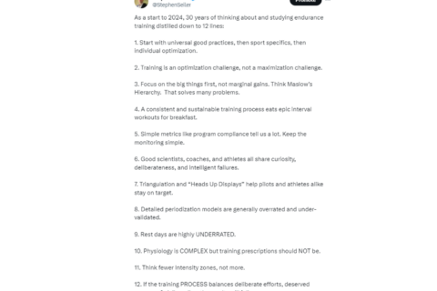
After 30 years of studying exercise endurance training, Dr. Seiler distills it all into 12 fundamental practices.

Please join or login to view this content.

Dr. Stephen Seiler

Related Posts